A long-travel axis rarely gets one magnet track. It gets a row of them, joined end to end, and a drawing that reads "linear Halbach array, full travel" is really a set of decisions about where the array is cut, what each cut has to keep, and who makes the joint. Those decisions cost nothing before tooling starts and a fixture rebuild after.
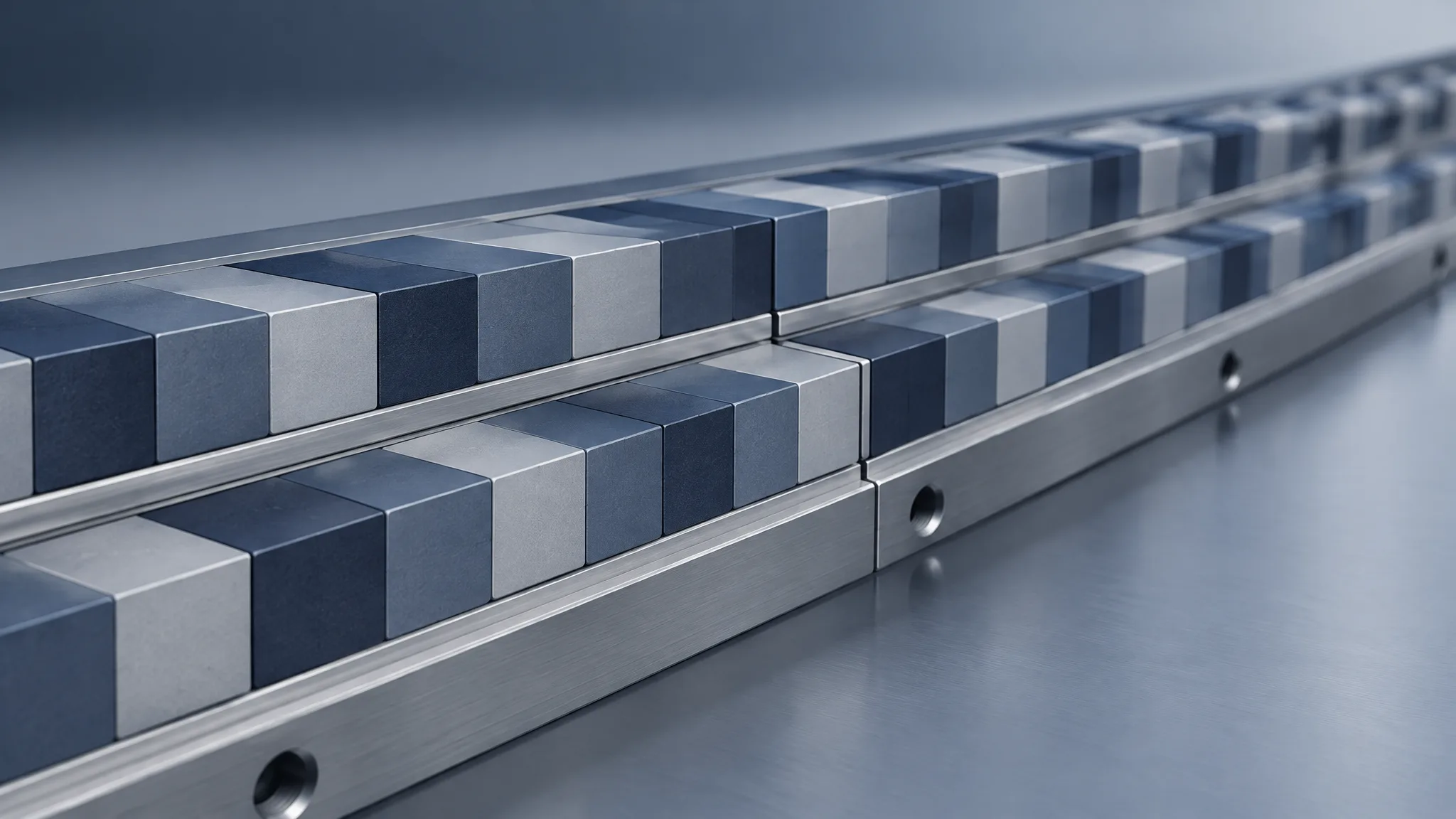
Our linear sections run from 10 mm to 600 mm and can be joined into longer travel, with magnets no thinner than 2 mm. What follows is how we would settle a joint on a track that has to stay one magnetic pattern across several sections.
How long is one linear Halbach array section?
As long as you can handle, and no longer than the build route allows — in our case 10 mm to 600 mm per section. The 600 mm end is where our single-section range stops, not where the magnetic pattern stops. Nothing in a Halbach sequence needs a break at a given length: the step from block to block continues across a joint exactly as it does inside a section, as long as the blocks on either side are placed as the next blocks of the sequence.
So the section length is a delivery unit, and it is set by things the field does not care about: what the assembly fixture can hold and keep square while the adhesive cures, whether the finished part has to pass through a magnetising cavity, and what can be packed, shipped and carried into the machine. That is why we settle it with whoever builds the track rather than on the machine drawing alone — a length chosen for the shipping crate can be one the fixture was never designed around.
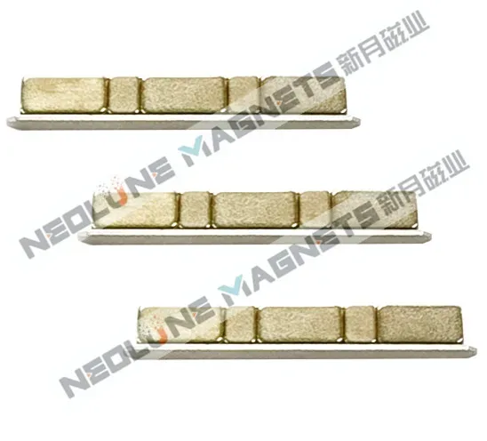
What does a splice have to keep?
Three separate things, measured three different ways: the magnetisation sequence, the pole pitch, and the mechanical joint. A joint that is mechanically tight can still be magnetically wrong, and a joint with a visible gap can still carry the pattern correctly.
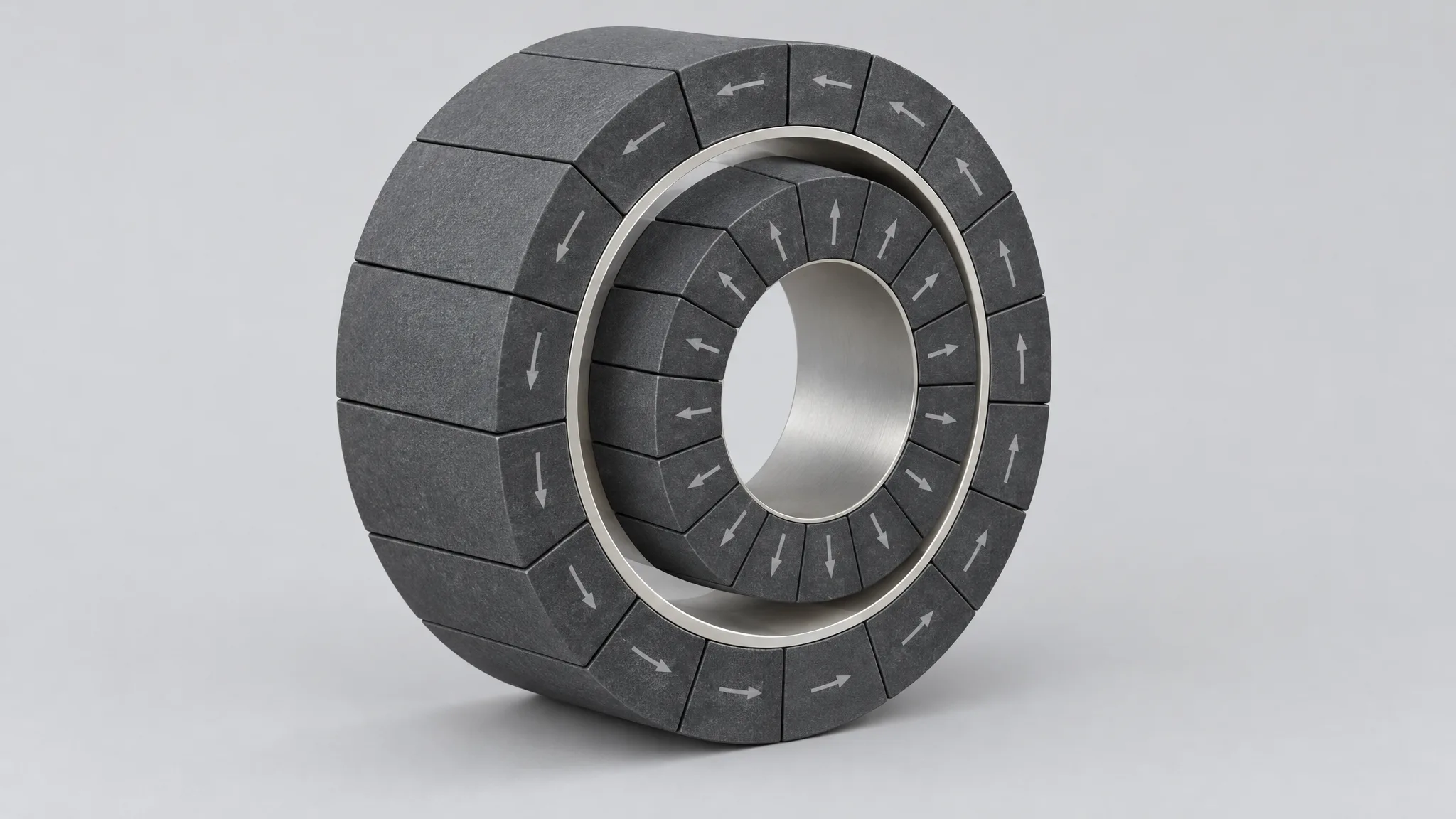
- The sequence. Each block is charged at an angle to its neighbour. At a joint the block after the seam has to be the next block of that sequence, not the first block of a new one. A joint where the pattern restarts, or where the last block is turned the wrong way, is a local defect in the working field, and it lands exactly where the coil crosses it.
- The pole pitch. The distance from the last pole centre before the joint to the first one after it belongs to the same pitch as the rest of the track. A gap between carriers is not the same quantity as pole-pitch error: a joint that measures acceptably can still carry a reversed end block or a field amplitude that does not match the section before it. A procurement guide published by another track supplier sets those quantities out separately for exactly that reason, and recommends scanning an assembled pair rather than one module at a time.
- The mechanical joint. The carrier-to-carrier gap, the step across the magnet faces and the flatness of the mounting face. A coordinate measuring machine can see these, which is why they tend to be specified first and the field second.
The field is not read at the magnet surface. It is read at the working gap where the coil runs, through a cover, a clearance and any encapsulation, so a joint that looks acceptable with a probe on the blocks can still be a problem at the plane that matters. We work from the target air-gap flux density for that reason.
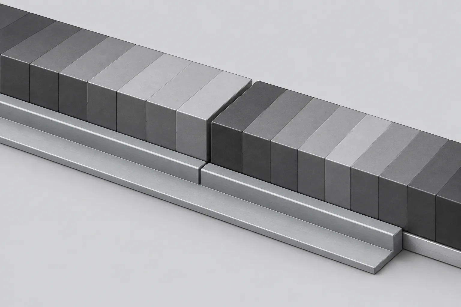
Who joins the sections — us or the machine builder?
Whichever the drawing says, because there is no default. It is one of the first questions a drawing review asks, and it changes three things at once.
If the sections are joined before delivery, the joint is made on our fixture, and the field evidence agreed for the order is taken from the joined assemblies before they ship as a longer magnetised rail. Long assemblies travel under magnetic shielding and protective packaging, because the transport risk is a chipped corner rather than a lost field — but a long rail is also a handling problem at the machine, and installation access often decides the length more than the build does.
If the sections are joined on the machine, each section is the unit that is made and checked, and the joint is made against the rail the customer provides. That route puts more weight on the drawing: the datum, the installation order and the field check through a joined pair have to be written down, or the joint is left to whoever is on site.
Neither route is better in the abstract. Joining before delivery concentrates the joint where the fixture and the scan are; joining on the machine keeps shipping and installation manageable and moves the risk to the interface. Say which one you want on the drawing, and add whether a section is interchangeable or the set is serialised and matched.
Where does the datum live: our carrier or your rail?
On a based track the datum is ours. The magnets are bonded to a carrier with its own mounting face and fastening holes, so the joint position, the reference face and the magnet face height are all features of the part you receive.
On a back-iron-free track the datum is yours. A Halbach pattern concentrates the field on the working face and works to cancel it behind — reduced rather than removed, since a finite array still leaks at its ends — and that lower backside field is what makes a heavy steel backing plate unnecessary. It also removes the stiff member that would otherwise carry the stack. The customer's housing or rail then has to locate the array and restrain it, so the reference faces that set each joint sit on your drawing, not ours. That is a structural decision as much as a magnetic one, and it belongs in the same review as the array design rather than at installation.
Both forms sit in the linear tracks and rings we build, and the drawing decides which one a project gets.
What holds the magnets at the joint while the adhesive cures?
A fixture, and the fixture is doing more of the work than the operator. On long tracks and large arrays the segments are magnetised first and bonded afterwards, because the finished part would have to fit a magnetising cavity and a long track does not; the blocks reach the fixture already repelling their neighbours, and the fixture holds them at the pitch and the angle while the adhesive cures. A complete ring that fits the cavity can be bonded first and magnetised afterwards, which takes the repulsion off the bench; which route a part gets follows its size, structure and batch quantity rather than a house rule.
For the large Halbach arrays we build we use UV and anaerobic adhesives, with assembly fixtures designed for batch assembly rather than one-off builds. The point is not the name on the adhesive bottle; it is that the local spacing at a joint is set by the tooling, so a joint settled on the drawing becomes a pocket in the fixture instead of an instruction to the person placing blocks. That is why we would rather review a joint before tooling than correct it afterwards: the drawing review and simulation step is where section length, joint position and assembly route are checked against each other.
What goes on the drawing at each joint?
Six things, and the last one is usually the one missing:
- Section length and section count, with the overall travel they have to cover.
- Joint position, dimensioned from one end datum along the travel, so positions do not accumulate through a chain of dimensions.
- Reference faces: the mounting face, the side alignment shoulder, and the magnet face height above the mounting face.
- End-block sequence at each joint — which block closes one section and which opens the next — so the magnetisation step is continued rather than restarted.
- Mechanical acceptance of the joint: the carrier-to-carrier gap, the step across the magnet faces and the flatness you will accept, taken from your axis error budget rather than from a default.
- The field check: at what plane and gap it is measured, on individual sections or through a joined pair, and what the report has to show.
We do not publish a straightness figure or a pole-pitch tolerance off the shelf. Our published envelope is the section range and the minimum magnet thickness; the numbers that decide whether a track is acceptable are agreed for the order, written on the drawing and measured the same way at both ends. Two builders can both call a track straight and mean different things, which is what the joint dimensions and the check are there to prevent.
What comes back with a long track?
Finished sections, or finished joined assemblies, packed with magnetic shielding and protection against chipping, together with the field evidence agreed for the batch. A three-dimensional field scan gives the air-gap flux density, how close the waveform comes to a sine and its harmonic content, and dimensional, magnetic-moment and coating checks sit alongside it. Which of those run, on how many parts and how often, is agreed per order — the scan proves the field and not the thrust, since force ripple and settling depend on the coil, the drive and the mechanics as well.
Send the drawing with the travel, the section length you can install, the joint positions, the target field at the working gap, the temperature and the quantity, and the array and its joints are reviewed together before anything is quoted. Paid samples start from one set, and the enquiry desk takes the drawing and the joint data; sales@neolune.com takes the files.